How To Find Change In Moment From A Position Time Graph

Section Learning Objectives

By the end of this section, you lot will be able to exercise the following:

• Explain the meaning of gradient in position vs. fourth dimension graphs
• Solve problems using position vs. fourth dimension graphs

Teacher Support

Instructor Support

The learning objectives in this section will assist your students principal the following standards:

• (4) Science concepts. The student knows and applies the laws governing motion in a variety of situations. The student is expected to:
  • (A) generate and interpret graphs and charts describing different types of motility, including the use of real-time technology such equally motion detectors or photogates.

Department Key Terms

dependent variable

independent variable

tangent

Teacher Support

Teacher Support

[BL] [OL] Draw a scenario, for example, in which yous launch a water rocket into the air. It goes upward 150 ft, stops, and then falls back to the earth. Accept the students assess the situation. Where would they put their zero? What is the positive management, and what is the negative direction? Have a pupil draw a film of the scenario on the board. And then draw a position vs. time graph describing the motion. Take students assistance you complete the graph. Is the line straight? Is it curved? Does information technology change management? What can they tell by looking at the graph?

[AL] Once the students have looked at and analyzed the graph, meet if they can depict different scenarios in which the lines would exist direct instead of curved? Where the lines would exist discontinuous?

Graphing Position equally a Function of Fourth dimension

A graph, like a picture, is worth a thousand words. Graphs not only incorporate numerical information, they as well reveal relationships betwixt physical quantities. In this section, we will investigate kinematics by analyzing graphs of position over fourth dimension.

Graphs in this text have perpendicular axes, i horizontal and the other vertical. When two physical quantities are plotted against each other, the horizontal axis is usually considered the independent variable, and the vertical axis is the dependent variable. In algebra, you lot would have referred to the horizontal axis as the ten-axis and the vertical axis as the y-centrality. As in Figure 2.x, a direct-line graph has the general form $y=m\mathrm{ten}+b$ .

Hither 1000 is the gradient, defined as the ascension divided by the run (equally seen in the effigy) of the straight line. The letter b is the y-intercept which is the point at which the line crosses the vertical, y-axis. In terms of a physical situation in the real world, these quantities will take on a specific significance, as we will see beneath. (Effigy 2.ten.)

Figure 2.10 The diagram shows a straight-line graph. The equation for the directly line is y equals mx + b.

In physics, time is normally the independent variable. Other quantities, such equally deportation, are said to depend upon information technology. A graph of position versus time, therefore, would accept position on the vertical axis (dependent variable) and time on the horizontal axis (independent variable). In this case, to what would the slope and y-intercept refer? Let'southward await back at our original example when studying distance and displacement.

The bulldoze to schoolhouse was five km from home. Let's presume it took 10 minutes to brand the drive and that your parent was driving at a constant velocity the whole time. The position versus time graph for this section of the trip would look like that shown in Effigy 2.11.

Figure two.11 A graph of position versus time for the drive to school is shown. What would the graph await similar if we added the return trip?

Equally we said earlier, d ₀ = 0 because we call home our O and start calculating from there. In Figure 2.11, the line starts at d = 0, as well. This is the b in our equation for a straight line. Our initial position in a position versus time graph is always the place where the graph crosses the x-axis at t = 0. What is the slope? The ascension is the change in position, (i.e., displacement) and the run is the change in fourth dimension. This relationship tin can as well be written

This human relationship was how we defined average velocity. Therefore, the gradient in a d versus t graph, is the average velocity.

Tips For Success

Sometimes, as is the example where we graph both the trip to school and the return trip, the behavior of the graph looks different during dissimilar time intervals. If the graph looks like a series of straight lines, then yous can calculate the average velocity for each time interval by looking at the slope. If y'all then desire to summate the average velocity for the entire trip, you lot can practise a weighted boilerplate.

Let'due south look at another example. Figure 2.12 shows a graph of position versus time for a jet-powered car on a very flat dry lake bed in Nevada.

Figure ii.12 The diagram shows a graph of position versus time for a jet-powered car on the Bonneville Table salt Flats.

Using the human relationship between dependent and independent variables, we see that the slope in the graph in Effigy 2.12 is average velocity, v _avg and the intercept is deportation at time zero—that is, d ₀. Substituting these symbols into y = mx + b gives

or

$$d=d_0+5t\text{.}$$

two.half dozen

Thus a graph of position versus fourth dimension gives a general relationship among deportation, velocity, and time, also equally giving detailed numerical information about a specific state of affairs. From the figure we tin can see that the car has a position of 400 m at t = 0 s, 650 k at t = ane.0 due south, and and so on. And we can learn well-nigh the object'southward velocity, every bit well.

Teacher Support

Instructor Back up

Instructor Demonstration

Help students learn what different graphs of deportation vs. time look like.

[Visual] Set up a meter stick.

1. If you can find a remote control machine, take i student record times every bit you send the car forward forth the stick, then backwards, then forrad again with a abiding velocity.
2. Take the recorded times and the change in position and put them together.
3. Get the students to coach you to draw a position vs. time graph.

Each leg of the journey should be a straight line with a different gradient. The parts where the car was going forrad should have a positive gradient. The part where it is going backwards would have a negative slope.

[OL] Inquire if the place that they accept equally nil affects the graph.

[AL] Is it realistic to draw whatever position graph that starts at residuum without some curve in information technology? Why might we be able to neglect the curve in some scenarios?

[All] Discuss what tin can be uncovered from this graph. Students should be able to read the net displacement, but they can likewise use the graph to decide the total distance traveled. And then enquire how the speed or velocity is reflected in this graph. Directly students in seeing that the steepness of the line (slope) is a mensurate of the speed and that the management of the slope is the direction of the movement.

[AL] Some students might recognize that a bend in the line represents a sort of slope of the gradient, a preview of acceleration which they will learn about in the adjacent affiliate.

Snap Lab

Graphing Motion

In this activity, y'all will release a ball downwards a ramp and graph the ball's deportation vs. fourth dimension.

• Choose an open location with lots of space to spread out and so there is less chance for tripping or falling due to rolling assurance.

• 1 ball
• ane board
• two or 3 books
• 1 stopwatch
• 1 tape mensurate
• 6 pieces of masking tape
• 1 piece of graph paper
• 1 pencil

Process

1. Build a ramp by placing 1 finish of the board on top of the stack of books. Adjust location, as necessary, until there is no obstruction along the straight line path from the bottom of the ramp until at least the next 3 m.
2. Marker distances of 0.5 m, 1.0 chiliad, i.v yard, 2.0 m, 2.5 m, and 3.0 m from the lesser of the ramp. Write the distances on the tape.
3. Have one person take the office of the experimenter. This person will release the ball from the summit of the ramp. If the brawl does not accomplish the iii.0 grand mark, then increase the incline of the ramp by adding another volume. Repeat this Pace as necessary.
4. Have the experimenter release the ball. Have a 2d person, the timer, begin timing the trial once the brawl reaches the bottom of the ramp and stop the timing one time the ball reaches 0.five m. Have a third person, the recorder, record the time in a data tabular array.
5. Repeat Step 4, stopping the times at the distances of 1.0 thousand, ane.v m, 2.0 m, 2.v m, and three.0 m from the bottom of the ramp.
6. Use your measurements of time and the deportation to brand a position vs. time graph of the ball'due south move.
7. Repeat Steps 4 through half-dozen, with different people taking on the roles of experimenter, timer, and recorder. Practice you get the same measurement values regardless of who releases the ball, measures the fourth dimension, or records the result? Discuss possible causes of discrepancies, if whatsoever.

True or Fake: The average speed of the ball volition be less than the average velocity of the ball.

1. True

2. Faux

Instructor Support

Teacher Support

[BL] [OL] Emphasize that the motion in this lab is the motion of the ball as it rolls along the floor. Ask students where in that location nil should exist.

[AL] Ask students what the graph would expect like if they began timing at the acme versus the bottom of the ramp. Why would the graph await dissimilar? What might account for the difference?

[BL] [OL] Take the students compare the graphs made with dissimilar individuals taking on dissimilar roles. Enquire them to determine and compare average speeds for each interval. What were the absolute differences in speeds, and what were the percent differences? Do the differences appear to be random, or are there systematic differences? Why might there be systematic differences between the two sets of measurements with dissimilar individuals in each role?

[BL] [OL] Accept the students compare the graphs made with different individuals taking on different roles. Enquire them to determine and compare average speeds for each interval. What were the accented differences in speeds, and what were the percent differences? Practice the differences announced to exist random, or are there systematic differences? Why might there be systematic differences between the two sets of measurements with dissimilar individuals in each function?

Solving Issues Using Position vs. Fourth dimension Graphs

So how practise we employ graphs to solve for things we want to know similar velocity?

Worked Example

Using Position–Fourth dimension Graph to Calculate Average Velocity: Jet Car

Find the average velocity of the car whose position is graphed in Figure one.13.

Strategy

The gradient of a graph of d vs. t is average velocity, since gradient equals ascent over run.

$$\text{slope =}\frac{\text{Δ}d}{\text{Δ}t}=\mathrm{five}$$

two.seven

Since the slope is constant here, any two points on the graph can be used to find the slope.

Discussion

This is an impressively high land speed (900 km/h, or virtually 560 mi/h): much greater than the typical highway speed limit of 27 m/s or 96 km/h, simply considerably shy of the tape of 343 m/southward or ane,234 km/h, prepare in 1997.

Teacher Support

Teacher Back up

If the graph of position is a directly line, then the but thing students need to know to summate the boilerplate velocity is the gradient of the line, rise/run. They tin utilize whichever points on the line are nearly convenient.

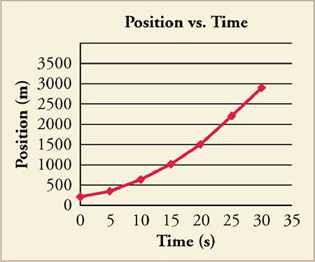
But what if the graph of the position is more than complicated than a directly line? What if the object speeds up or turns around and goes backward? Can we effigy out anything virtually its velocity from a graph of that kind of motility? Let's take some other look at the jet-powered car. The graph in Figure ii.13 shows its motion as it is getting up to speed later on starting at rest. Fourth dimension starts at zero for this motility (as if measured with a stopwatch), and the displacement and velocity are initially 200 one thousand and 15 g/s, respectively.

Figure 2.xiii The diagram shows a graph of the position of a jet-powered automobile during the time span when it is speeding upwardly. The gradient of a distance versus time graph is velocity. This is shown at two points. Instantaneous velocity at any point is the slope of the tangent at that signal.

Figure 2.14 A U.Southward. Air Strength jet auto speeds down a runway. (Matt Trostle, Flickr)

The graph of position versus time in Figure 2.thirteen is a bend rather than a straight line. The slope of the curve becomes steeper every bit fourth dimension progresses, showing that the velocity is increasing over time. The slope at any point on a position-versus-fourth dimension graph is the instantaneous velocity at that point. Information technology is institute by drawing a straight line tangent to the curve at the point of interest and taking the slope of this straight line. Tangent lines are shown for two points in Figure 2.13. The average velocity is the cyberspace deportation divided by the time traveled.

Worked Instance

Using Position–Time Graph to Summate Boilerplate Velocity: Jet Car, Take Two

Calculate the instantaneous velocity of the jet machine at a time of 25 s by finding the slope of the tangent line at bespeak Q in Figure 2.13.

Strategy

The slope of a curve at a indicate is equal to the slope of a straight line tangent to the curve at that point.

Discussion

The entire graph of v versus t can be obtained in this style.

Teacher Support

Teacher Back up

A curved line is a more complicated instance. Define tangent as a line that touches a curve at just one point. Testify that equally a directly line changes its angle next to a bend, it actually hits the bend multiple times at the base, but simply ane line will never touch at all. This line forms a right bending to the radius of curvature, but at this level, they can just kind of eyeball information technology. The slope of this line gives the instantaneous velocity. The well-nigh useful part of this line is that students can tell when the velocity is increasing, decreasing, positive, negative, and zero.

[AL] You could find the instantaneous velocity at each signal along the graph and if you graphed each of those points, you would accept a graph of the velocity.

Practice Issues

sixteen .

Calculate the average velocity of the object shown in the graph beneath over the whole time interval.

1. 0.25 m/south
2. 0.31 m/s
3. three.ii grand/s
4. 4.00 m/s

17 .

Truthful or Fake: By taking the gradient of the curve in the graph you can verify that the velocity of the jet car is 125\,\text{m/s} at t = twenty\,\text{south}.

1. True

2. False

Check Your Agreement

18 .

Which of the following information about motion can exist determined past looking at a position vs. fourth dimension graph that is a straight line?

1. frame of reference
2. average dispatch
3. velocity
4. direction of strength applied

19 .

True or False: The position vs time graph of an object that is speeding upwards is a straight line.

1. True

2. Imitation

Teacher Support

Teacher Support

Use the Check Your Understanding questions to appraise students' achievement of the section'southward learning objectives. If students are struggling with a specific objective, the Check Your Agreement will assistance identify direct students to the relevant content.

Source: https://openstax.org/books/physics/pages/2-3-position-vs-time-graphs

Posted by: hiersmorgilizeed.blogspot.com

Share this post